Image-Based Meta-Analysis (Beta)

A PRISMA workflow for a meta-analysis about reward

It's finally arrived after years of patience -- Image Based Meta-Analyses. Well, almost, it's in Beta so we haven't made all the knobs accessible yet, but enough knobs to do some legitimate work. This tutorial builds a complete image-based meta-analysis (IBMA) end to end: 16 candidate studies found, 12 retained through PRISMA screening and eligibility, 19 statistical maps selected, and a Stouffers meta-analysis run in the cloud.

I'm assuming many of you are familiar with the general workflow of a CBMA; so I will place emphasis on the steps where IBMA differs from coordinate-based meta-analysis (CBMA). The curation flow will look familiar — but some steps are meaningfully different. They are flagged ▲ IBMA-SPECIFIC below.

---

0. CBMA vs IBMA: poor and big data versus rich and small data

A CBMA takes the peak coordinates a paper reports — a handful of (x, y, z) rows that survived the authors' threshold. An IBMA takes the whole statistical map: every voxel, including the sub-threshold ones. IBMA therefore uses far more of each study's evidence, and can combine effect sizes rather than merely testing whether reported peaks cluster in space.

The cost is availability. Measured against the live NeuroStore database on the day this tutorial was written (08/23/2026):

	CBMA	IBMA
Unit of input	peak coordinate table	whole-brain statistical map
Studies available in NeuroStore	32,438	684 (~47× fewer)
Does the statistic type matter?	No	Yes, decisively
Thresholded input	inherent — peaks are thresholded	disqualifying
Selection granularity	per analysis	per image
Estimators offered	ALE, ALESubtraction, KDA, MKDAChi2, MKDADensity	Fishers, Stouffers
Missing-coverage handling	n/a	aggressive_mask
Typical runtime (measured)	~3 min / 554 analyses	~4 min / 19 images; >73 min / 746 images

That last row is the practical reason this tutorial uses 19 maps and not 750.

Which statistic types can be used?

Fishers and Stouffers both require z maps. But you can input other statistic types — Compose can derive it:

z  ←  p
z  ←  t + sample_size

That matters enormously for how much data you can reach. Filtering the image studies by statistic type gives:

map_type	Studies
any	684
z	129
t	390
beta_variance	0

So accepting t maps roughly triples your candidate pool. Two caveats worth knowing:

• beta_variance is empty across the entire database. This is why Compose exposes only Fishers and Stouffers today: the config file defines nine IBMA estimators, and the other seven (DerSimonianLaird, Hedges, WeightedLeastSquares, VarianceBasedLikelihood, PermutedOLS, SampleSizeBasedLikelihood, FixedEffectsHedges) require beta+varcope or bare t, for which there is no data. The two-estimator menu is a response to the data, not an arbitrary limit.
• There is no beta+varcope → z path, even though t = β/√varcope is elementary. The derivation graph only reaches t from (p, sample_size) or (sample_size, z).

This tutorial uses map_type = z to keep the worked example simple. For real work, run it twice — once with z, once with t — and compare what each pool gives you.

---

1. Create an IBMA project

NEW PROJECT → choose IBMA → CREATE NEW PROJECT.

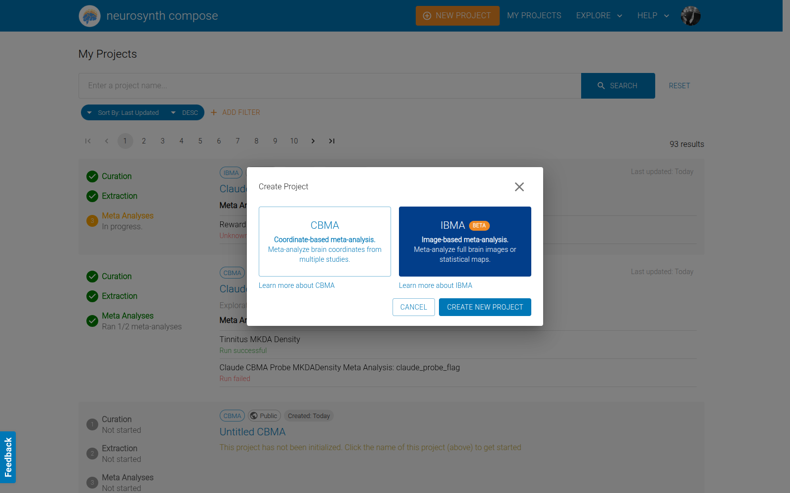
Note the BETA chip. Pick deliberately: the project type determines which estimators you are offered later and cannot be changed afterwards.

Give the project a name and description by clicking the pencil icons.

---

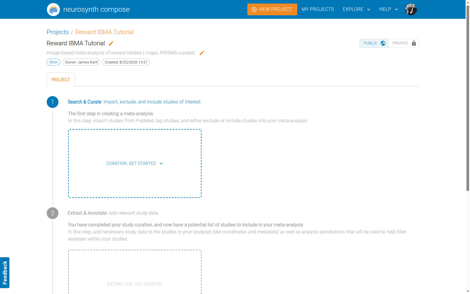
2. Choose the PRISMA workflow

CURATION: GET STARTED opens a two-option menu.

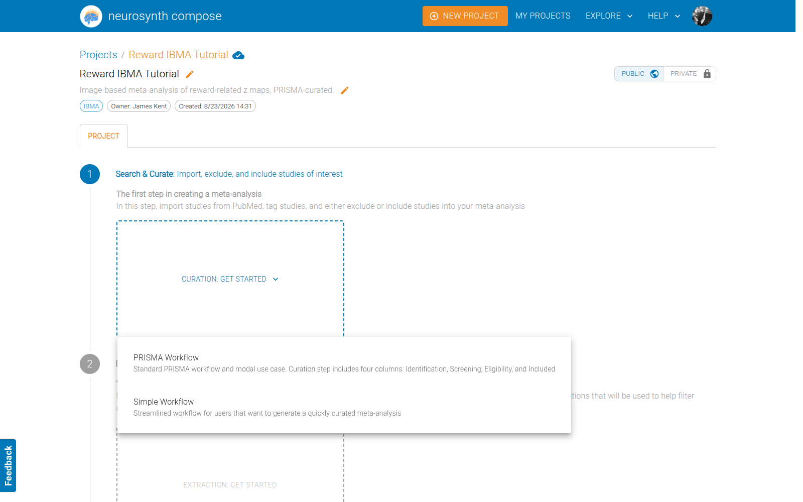
• Simple — two columns (Unreviewed → Included). Fine for exploratory work.
• PRISMA — four columns (Identification → Screening → Eligibility → Included), which is what you need if the result is going into a paper.

Choose PRISMA Workflow. This choice is structural and, as far as the UI exposes, not reversible — so decide before importing.

---

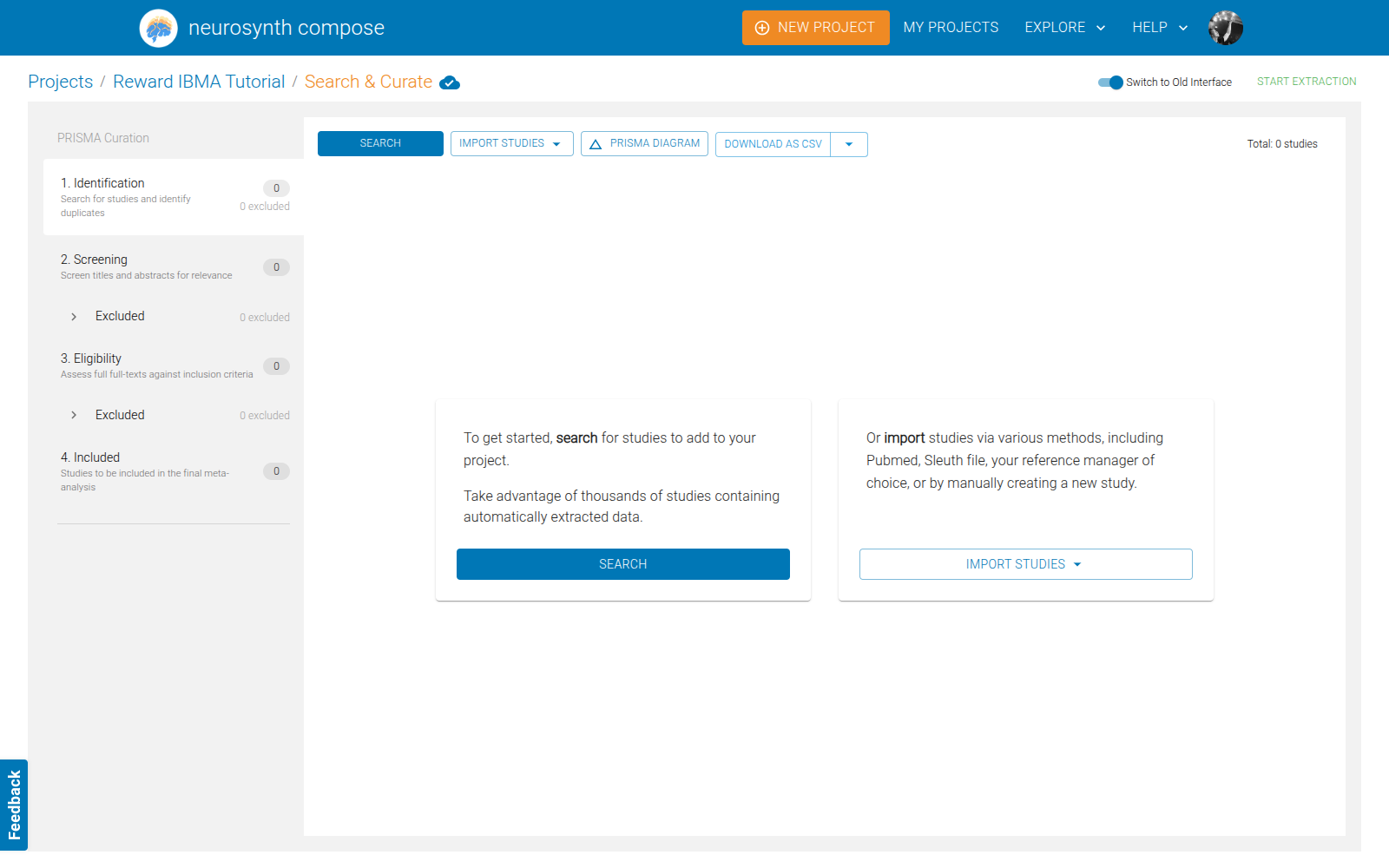
3. ▲ IBMA-SPECIFIC — Search with the Map Type filter

Click SEARCH. Two things are already different from a CBMA project:

• Study Data Type defaults to Images, not Coordinates.
• A Map Type chip appears. This control exists only for IBMA projects.

Open it:

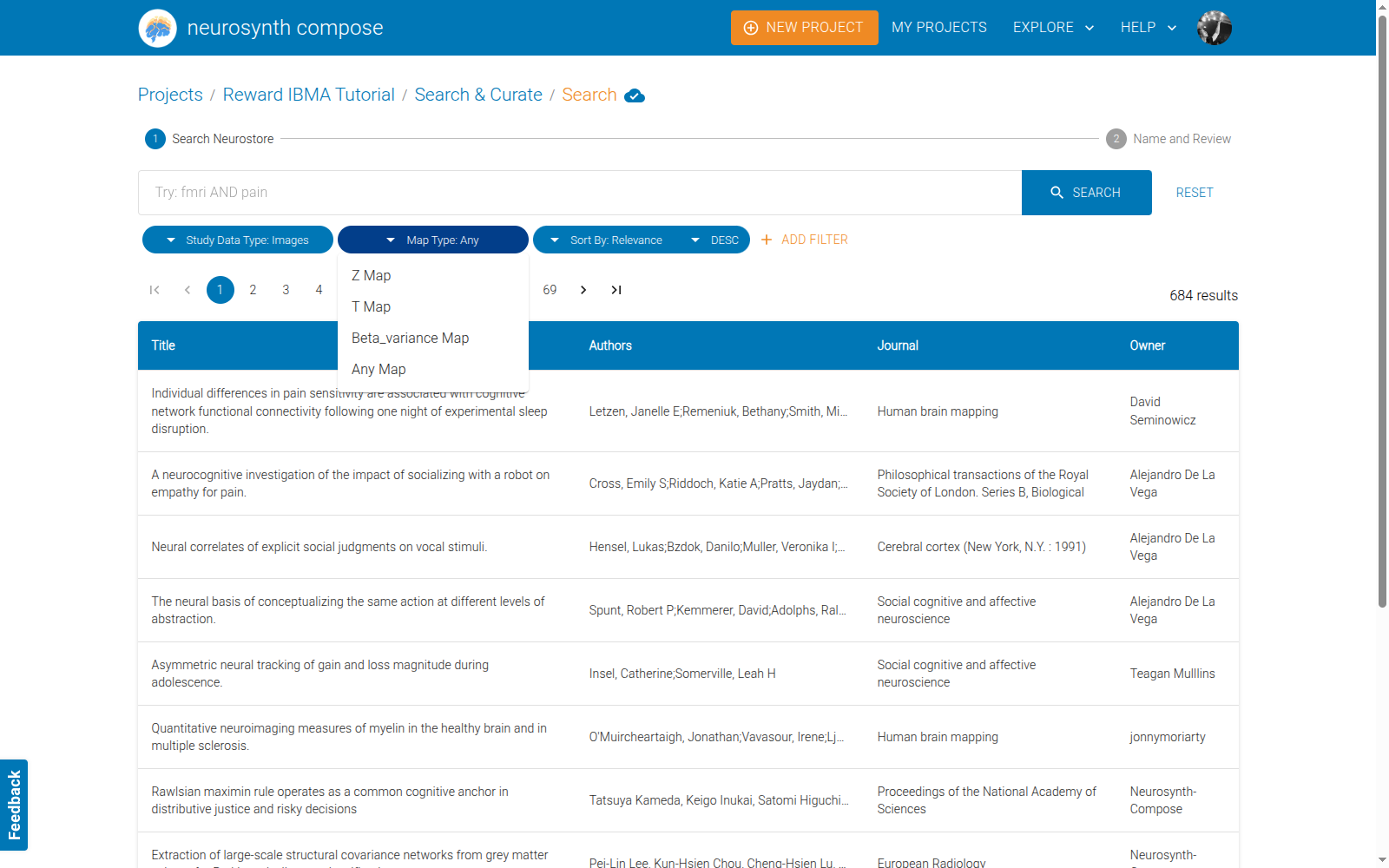
Z Map / T Map / Beta_variance Map / Any Map. This is the single most important control in the IBMA workflow and it defaults to Any, which will hand you anatomical templates, ROI masks and F maps alongside usable data. Sometimes people label the data incorrectly, so using Any will be more comprehensive.

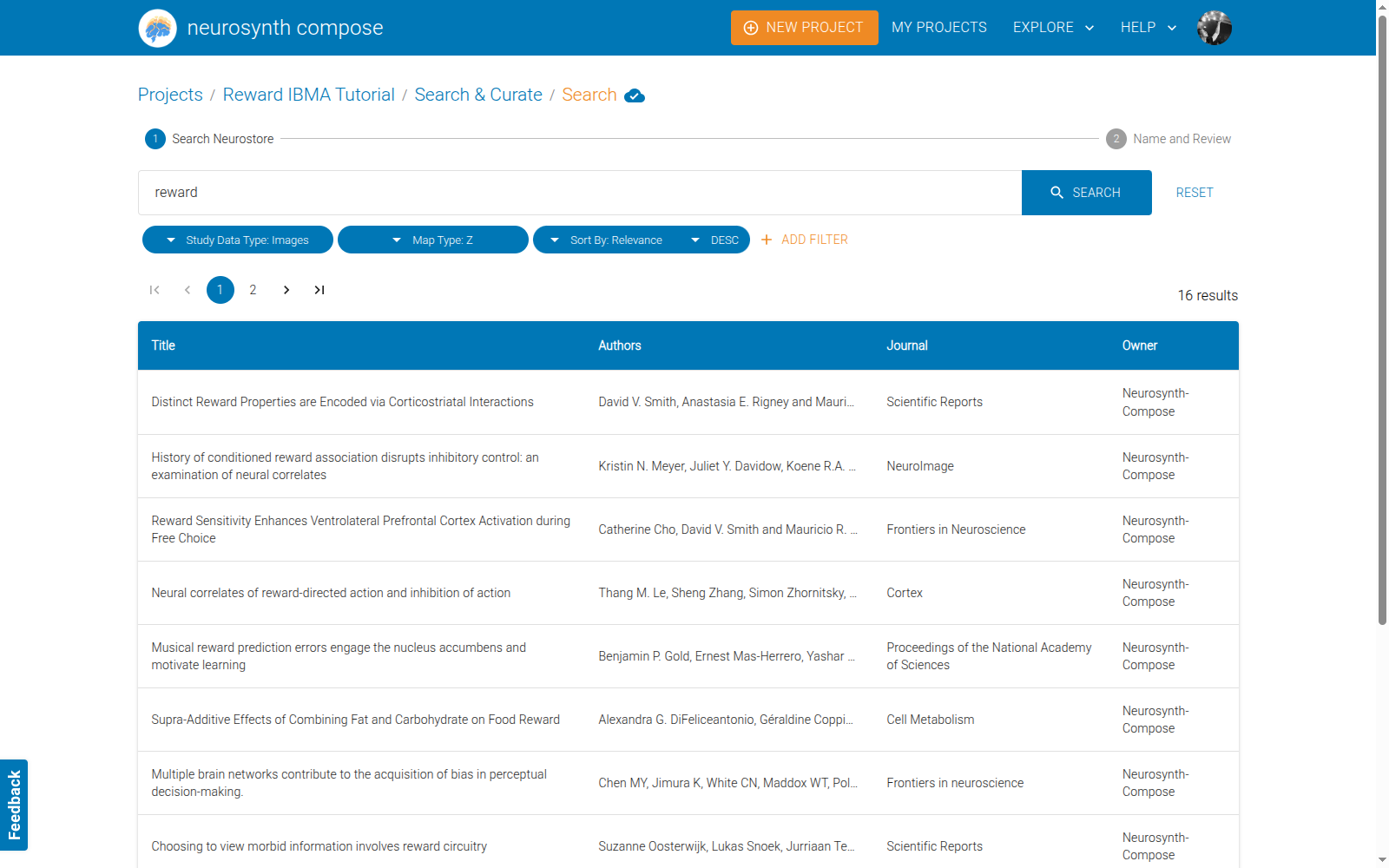
For this tutorial, we are going to use Z Map to keep the example simple. Select Z Map, type reward, and search. Result: 16 studies.

---

4. Name and review the import

Click NEXT. Name the import something that records your query — future-you will want to know exactly what produced this set. We do our best to preserve the query in the import name, but if you want to name it something else, do so here.

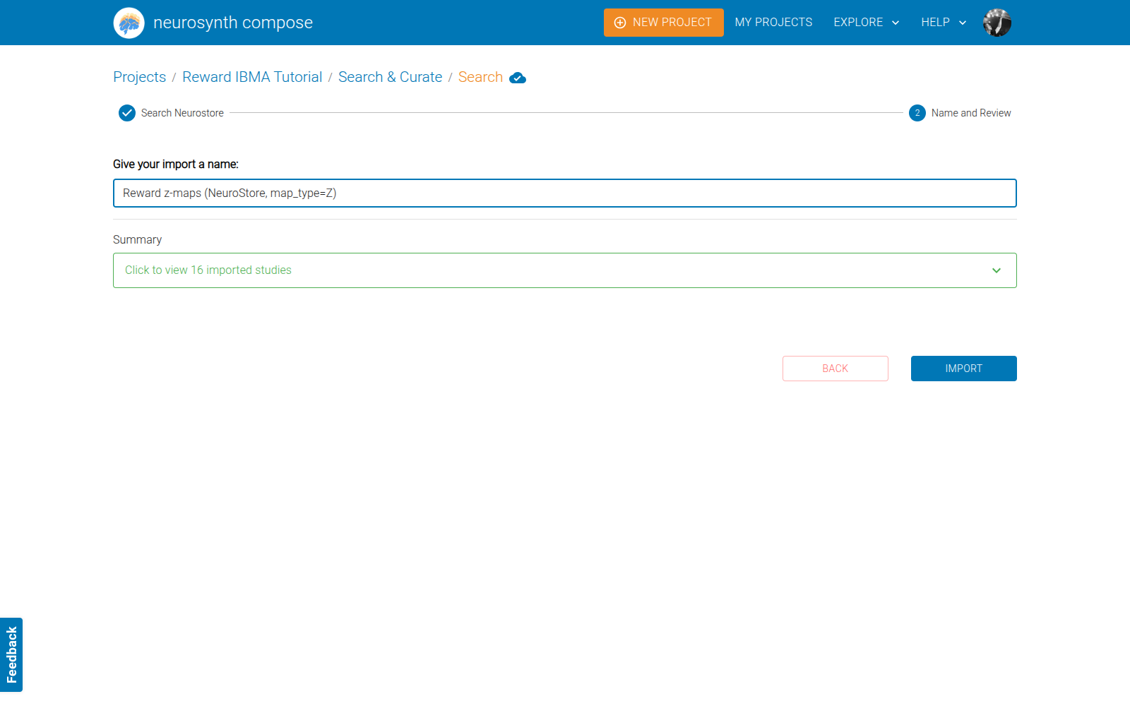
Expanding the summary lists every study with view study in neurostore / view study in pubmed / view full article links. This is the fastest way to sanity-check a search before committing to it. Click IMPORT.

---

5. Identification

The 16 studies land in Identification, and Compose checks for duplicates across all imports in the project.

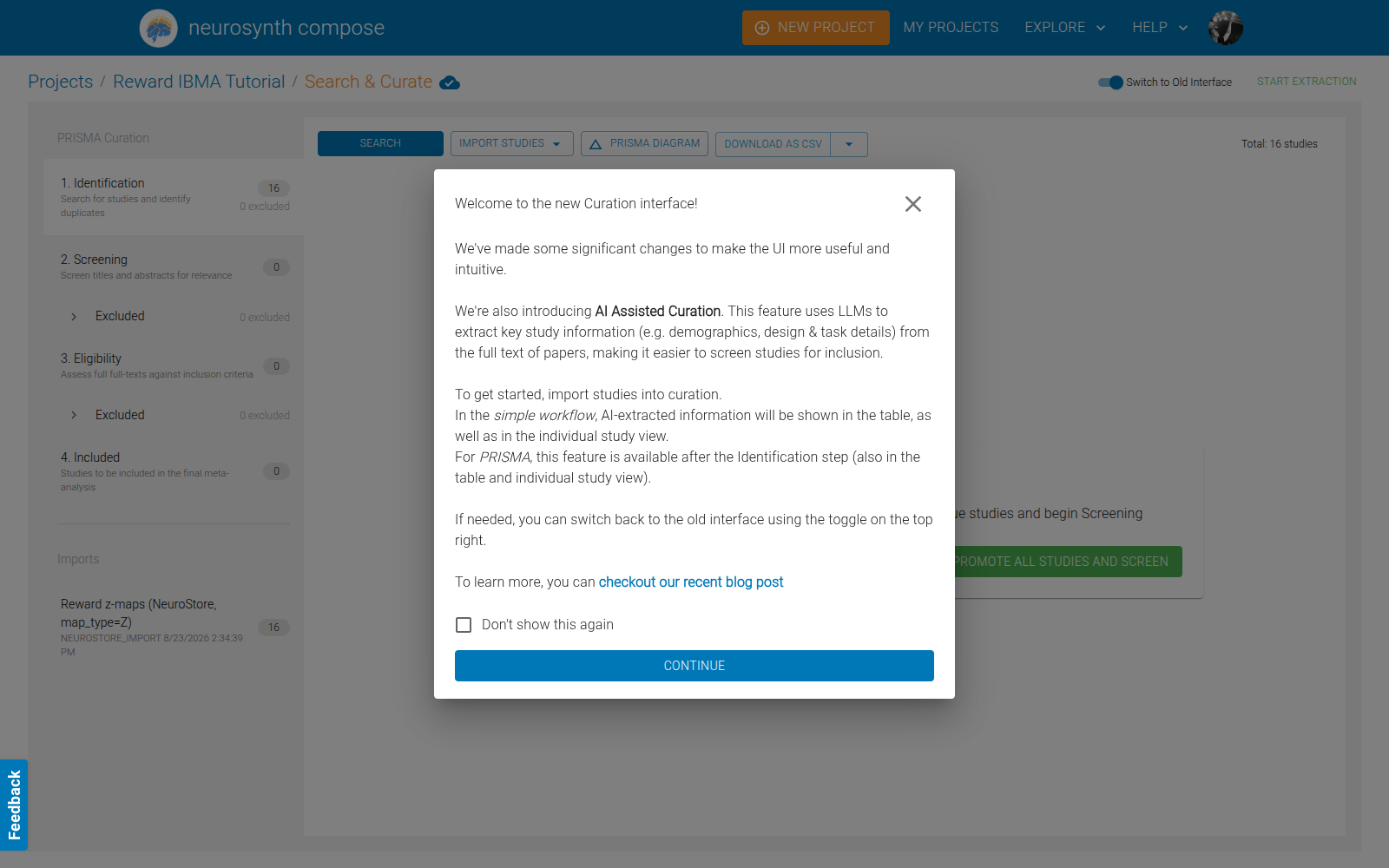
With a single import there are none. If you had imported "reward" and "reinforcement" separately, duplicates would be detected here and excluded automatically — and correctly un-excluded if you later delete one of the imports.

Click PROMOTE ALL STUDIES AND SCREEN.

---

6. Screening — title and abstract

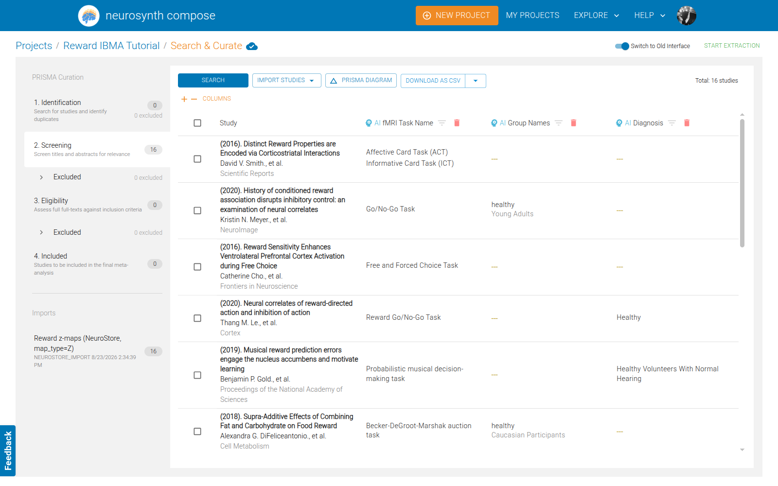
Screening is the ordinary PRISMA step: decide from the title and abstract whether the study addresses your question. Nothing IBMA-specific here.

Select a row with its checkbox. The action bar appears.

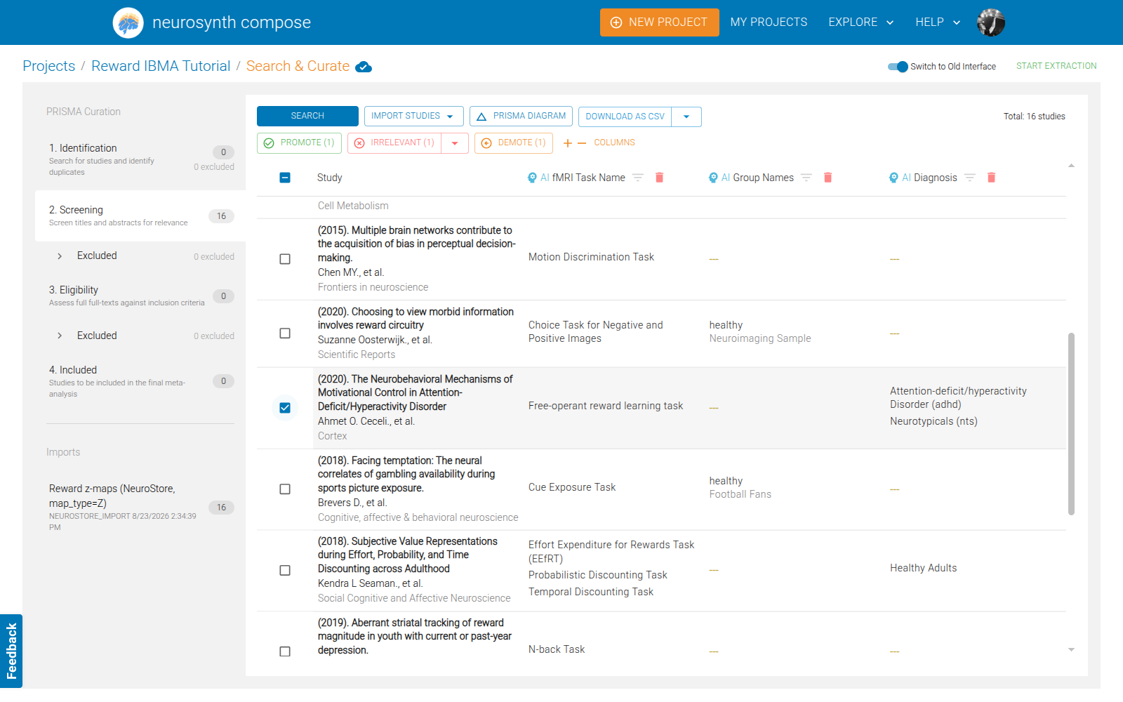
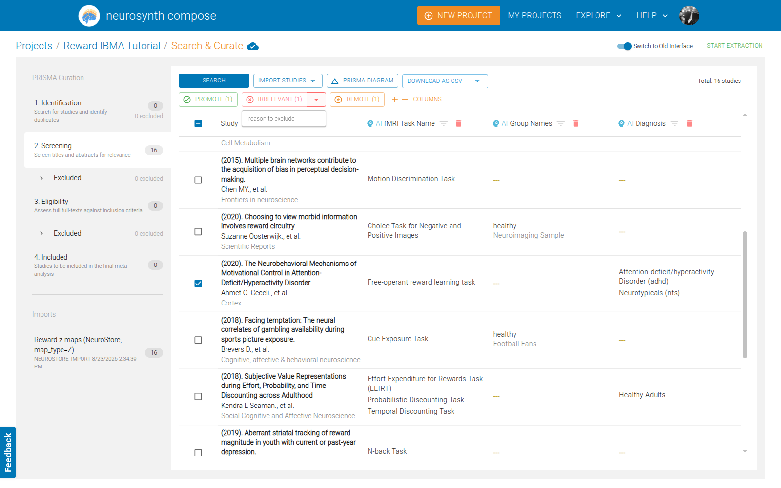
Clicking IRRELEVANT directly records the generic reason "Irrelevant". Use the small caret beside it instead — it opens a free-text box where you can create a specific reason, which becomes a labelled box in your PRISMA diagram.

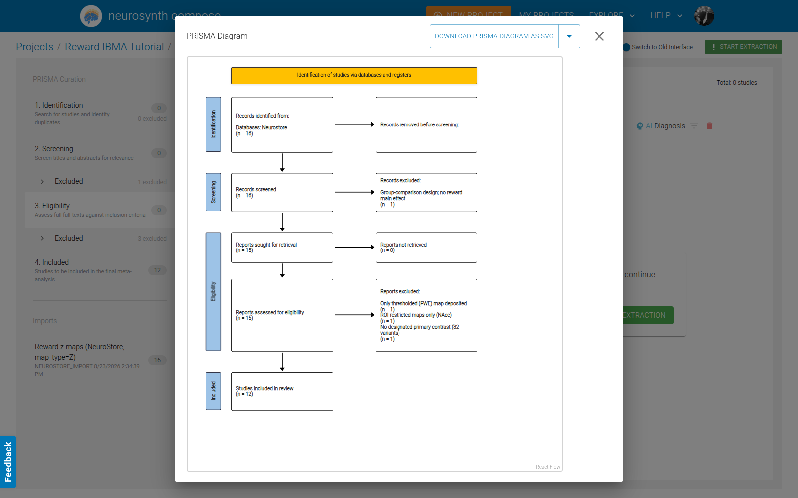
In this run, one study was excluded here:

Study	Reason
The Neurobehavioral Mechanisms of Motivational Control in ADHD (2020)	Group-comparison design; no reward main effect

Its design is clear from the abstract: every map is an ADHD-vs-control contrast, so there is no group-level reward effect to contribute. 15 studies proceed. Select all and PROMOTE.

---

7. Eligibility — full text assessment

Currently, you can only assess eligibility from the full text; checking for method designs, what contrasts were actually analyzed, etc. We may decide to add links to the corresponding neurovault collection, so you can assess whether the image corresponding to the contrast you want is actually available. For now, that will be decided during the extraction step.

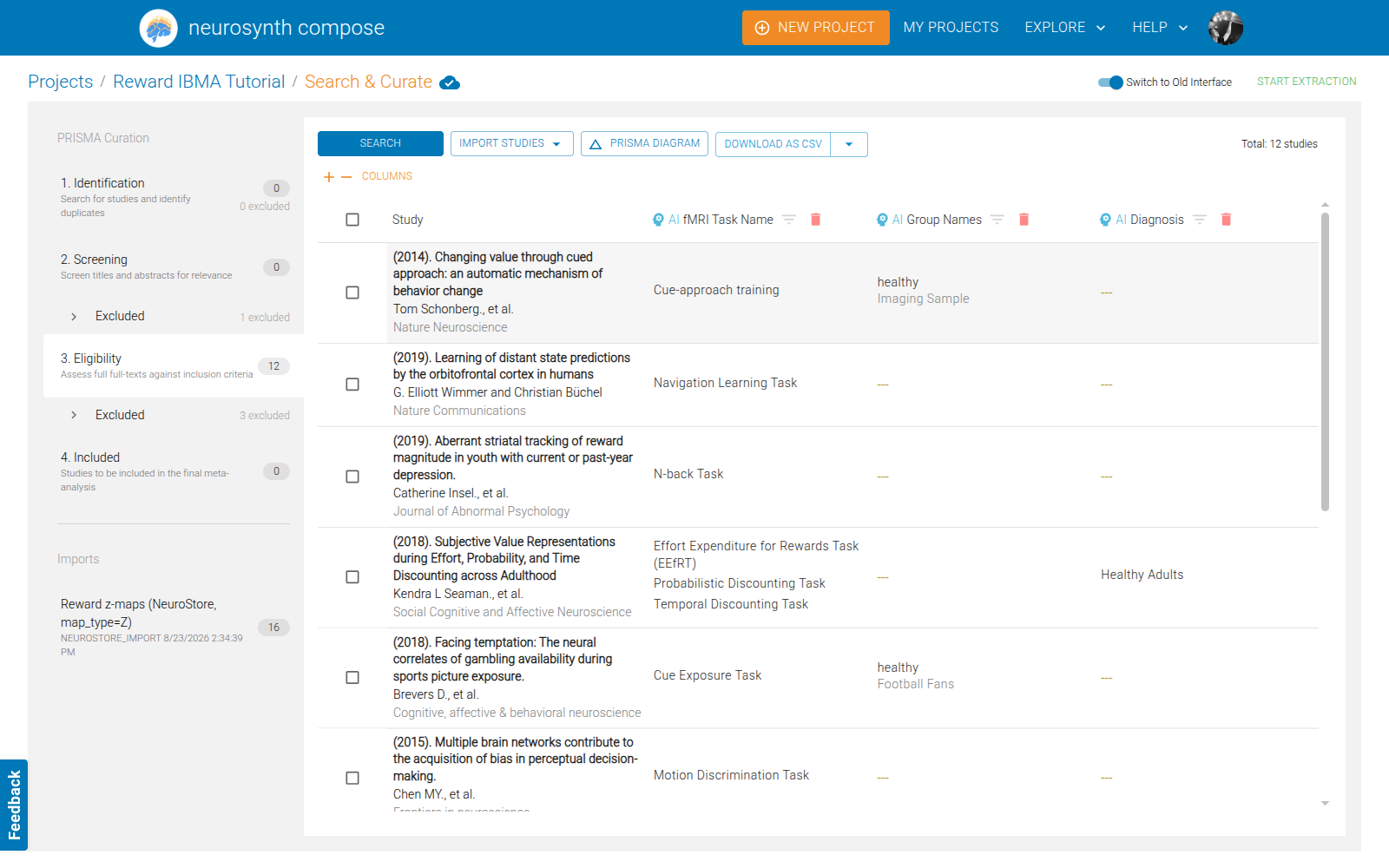
12 studies remain. Select all and INCLUDE.

---

8. The PRISMA diagram

PRISMA DIAGRAM renders the flow, with your custom reasons as labelled boxes.

---

9. Extraction — build the studyset

START EXTRACTION → step through the wizard → START. Compose creates a studyset from your 12 included studies, ingests anything new into NeuroStore, and creates a default included annotation column.

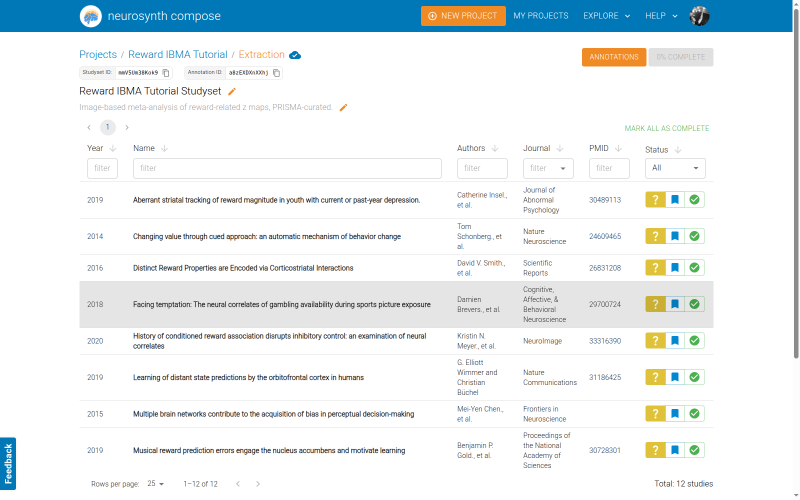
A note on versions. A NeuroStore study can have several versions, and they do not all contain the same images. Four of the twelve studies here carry z maps only in one of three of the available versions.

---

10. ▲ IBMA-SPECIFIC — Choose the images

This is the heart of an IBMA and it has no CBMA counterpart.

Your 12 studies contain 77 analyses, and by default the included column marks every one of them true. Left alone, your meta-analysis would pool all 77 — including PPI connectivity maps, thresholded/unthresholded duplicates of the same contrast, and F maps.

Open any study to see what you are actually choosing between.

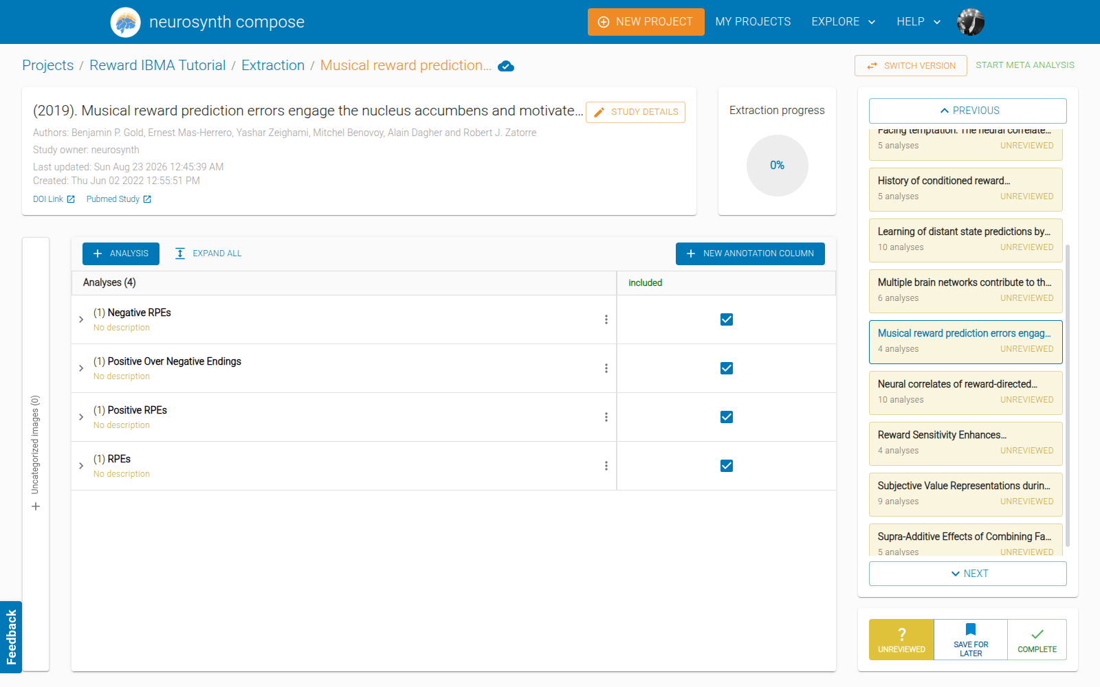
Uncheck everything that is not a contrast you want. Three rules:

1. Prefer unthresholded. Where a study deposits both, e.g. thresh affective and unthresh affective, always choose the unthresholded one.
2. One inference type. Do not pool activation maps with PPI/connectivity maps; they test different things. In this set, 5 of one study's 10 analyses are PPI.
3. Never include both signs of the same contrast. "betting minus watching" and "watching minus betting" are the same map negated; including both cancels to zero. Don't do that if you want a result from the meta-analysis.

On rule 3's flip side: where a paper offers several equally defensible contrasts and no principled way to choose, keeping more than one is better than guessing. Forcing a single pick substitutes your judgement for the data, and the statistical cost of keeping several is lower than you might expect — NiMARE automatically corrects the variance for contrasts that share a study (see caveat 2 in §14). Six of the twelve studies here contribute two or three contrasts for exactly this reason.

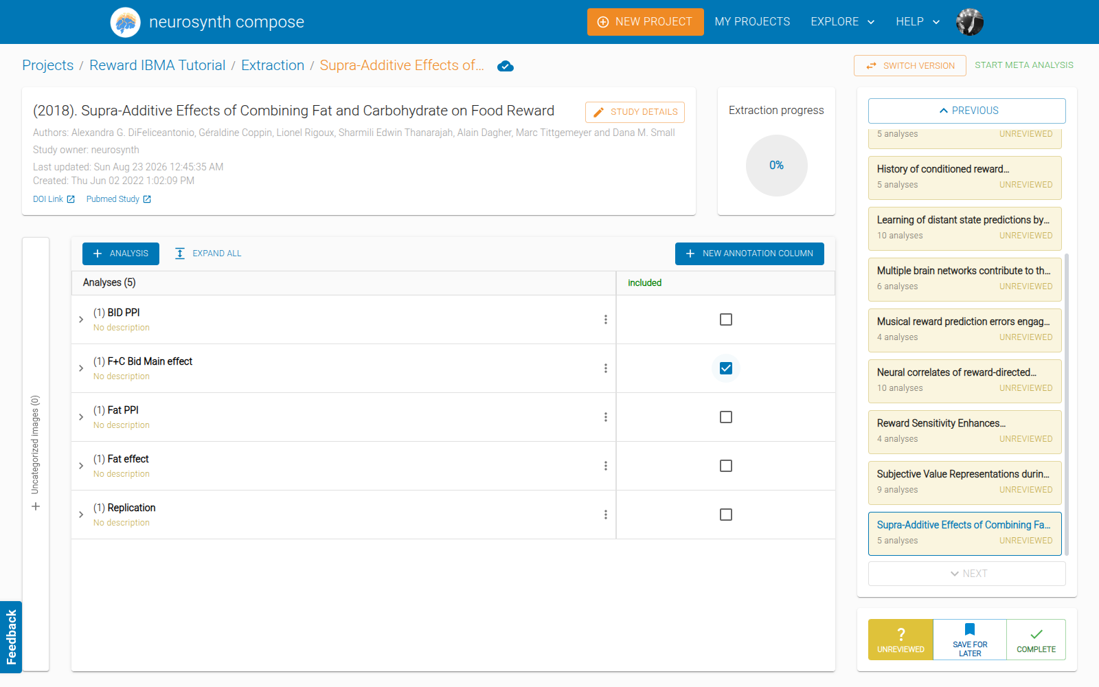
The final selection — 19 images from 12 studies:

Study (year)	Images	Contrast(s) kept
Subjective Value during Effort/Probability/Time Discounting (2018)	3	Subjective Value during Effort / Probability / Temporal Discounting
Distinct Reward Properties via Corticostriatal Interactions (2016)	2	unthresh affective, unthresh informative
Multiple brain networks … acquisition of bias (2015)	2	context-based / context-free action reward error
History of conditioned reward association (2020)	2	Rewarded > Unrewarded No-go; Rewarded > Unrewarded False Alarm
Neural correlates of reward-directed action (2020)	2	GS dollar RT > GS control RT; NGS dollar > nickel rate
Changing value through cued approach (2014)	2	Fig3A_zstat1, Fig3B_zstat1
Reward Sensitivity Enhances vlPFC Activation (2016)	1	Figure2 Free vs Forced TEPS unthresh
Musical reward prediction errors (2019)	1	RPEs
Facing temptation: gambling availability (2018)	1	"betting minus watching"
Aberrant striatal tracking of reward magnitude (2019)	1	gain > loss, mean across HC and MDD
Learning of distant state predictions by OFC (2019)	1	Reward
Supra-Additive Effects of Fat and Carbohydrate (2018)	1	F+C Bid Main effect

danger

A failure mode worth knowing. A study can silently drop to zero included images and nothing warns you — the run simply proceeds with fewer studies than you intended. This happened during this tutorial: one analysis is named F+C Bid Main effect with a double space, which the browser collapses to one when displayed. Always confirm the N / 77 analyses selected figure on the Review screen matches your intent.

---

11. Specify the meta-analysis

META-ANALYSIS SPECIFICATION → choose an estimator.

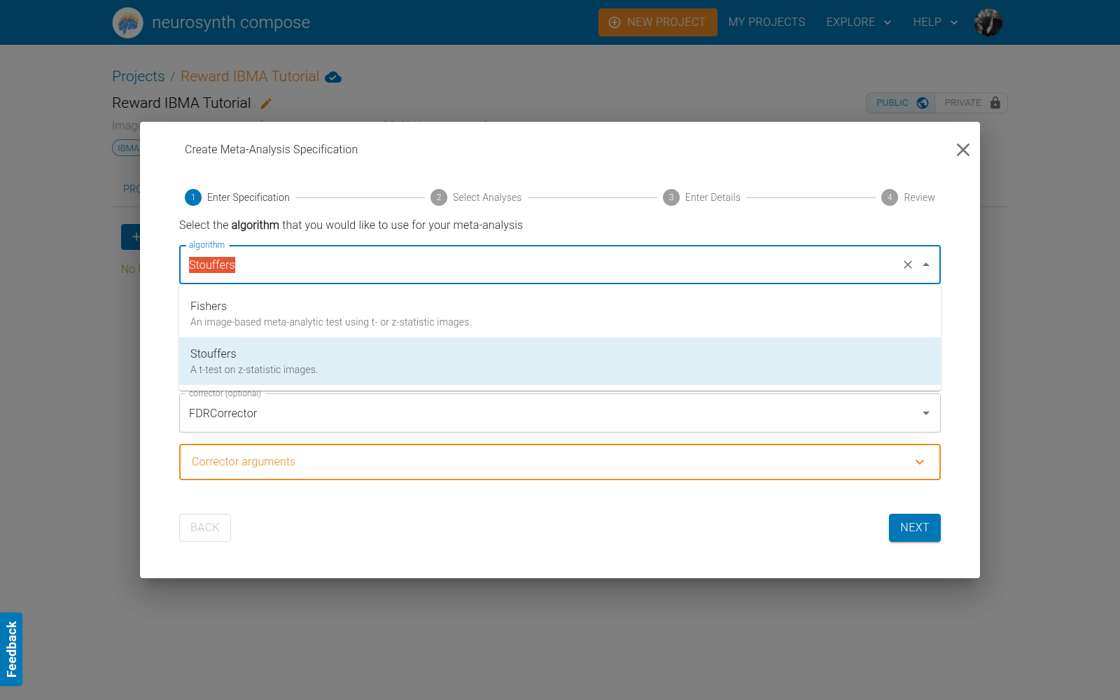
• Stouffers — a t-test on z-statistic images. Used here.
• Fishers — combines p-values derived from t or z images. More sensitive to a single strong study; Stouffers weights studies more evenly.

Leave the corrector at FDRCorrector (alpha=0.05, method=indep). FDR is the only option currently enabled for IBMA.

Three Stouffers arguments deserve attention, and two of them have no CBMA analogue:

• aggressive_mask (default False) — ▲ IBMA-specific. Studies differ in brain coverage. True analyses only voxels present in every map (a strict intersection); False runs per-voxel analyses on whatever subset of studies has valid data there. False keeps more brain but means different voxels rest on different numbers of studies.
• two_sided (default True) — tests for both increases and decreases.
• use_sample_size — weighted Stouffer's. Sample sizes are present in NeuroStore (analysis.metadata.sample_size; 17–88 in this set), so this is usable — but note it weights by n, which will amplify any over-weighting from studies contributing several contrasts.

Click NEXT. Verify the count.

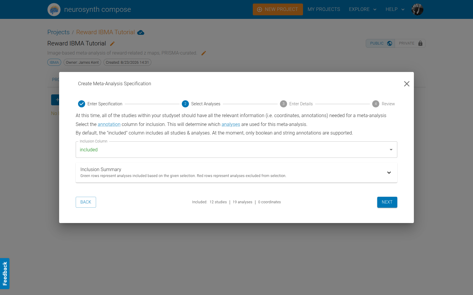
Included: 12 studies | 19 analyses | 0 coordinates

Name it, then check the Review screen.

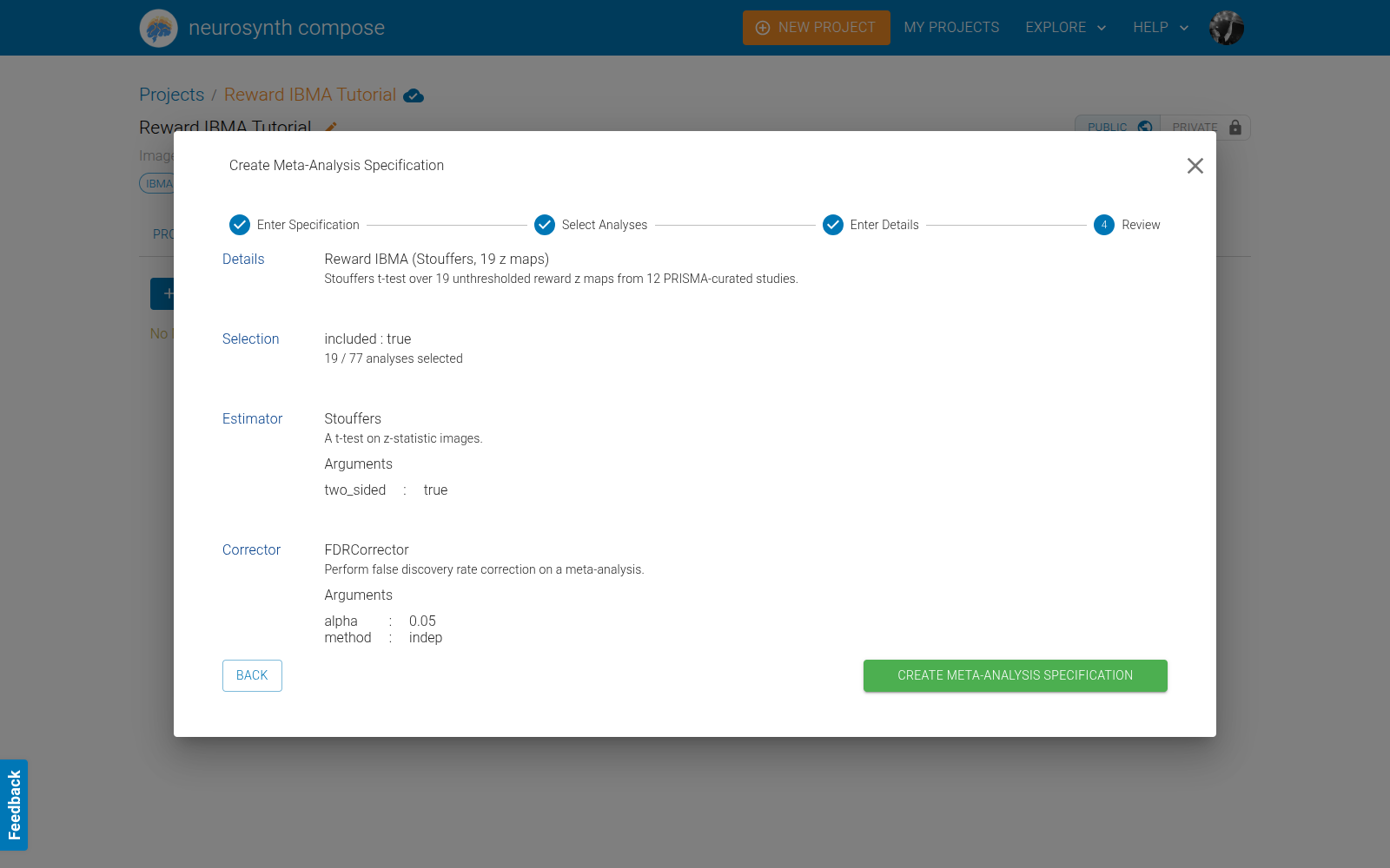
19 / 77 analyses selected — this is the number to verify before creating.

---

12. Run

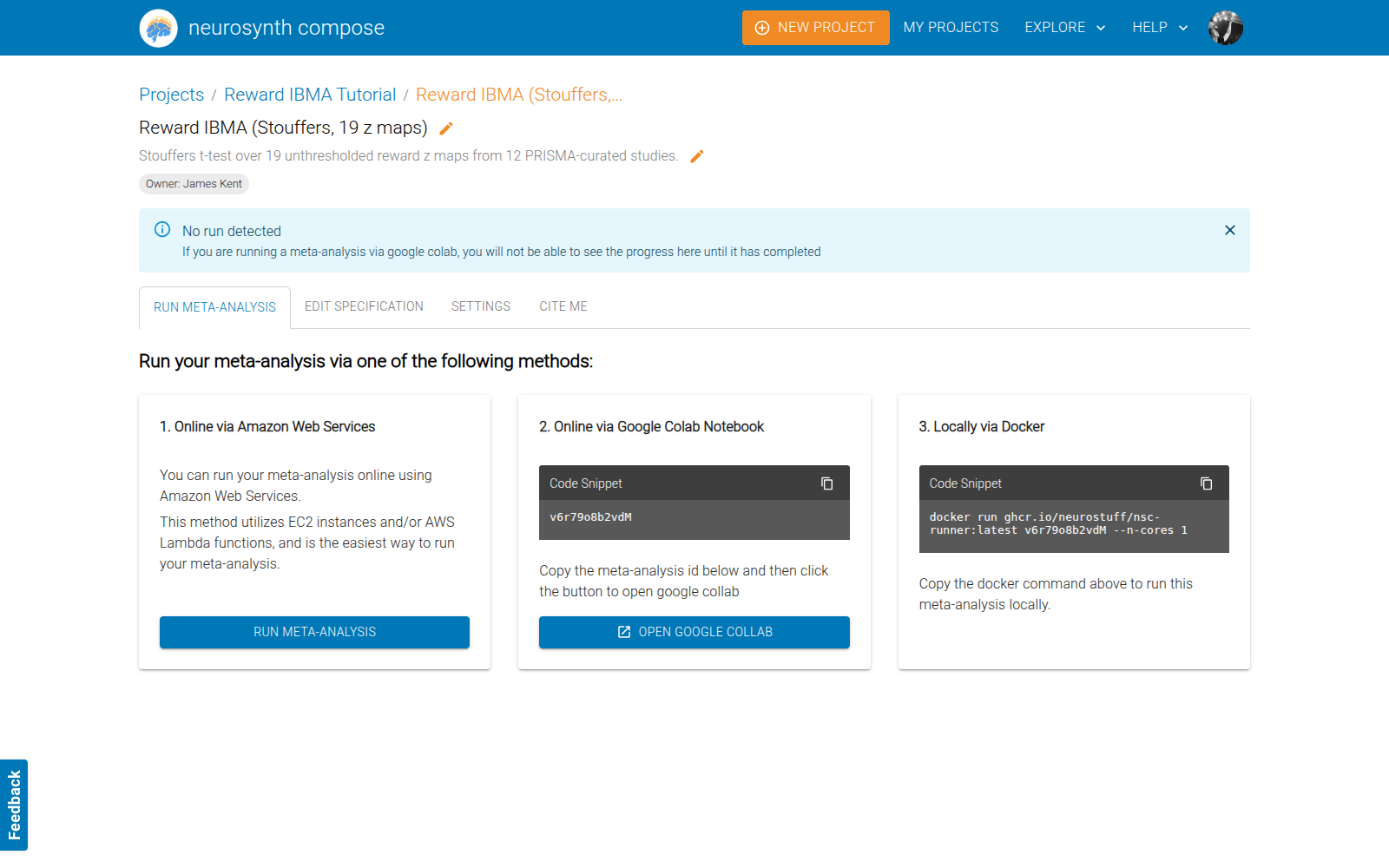
Three execution routes: AWS (one click), Google Colab, or locally via docker run ghcr.io/neurostuff/nsc-runner:latest <id> --n-cores 1.

Use AWS for this. Nineteen images completed in about four minutes. For scale: a run with 746 images was still going after 73 minutes, having emitted a single log line — so if you are working at that size, prefer the Docker route, where you can actually watch progress.

---

13. Results

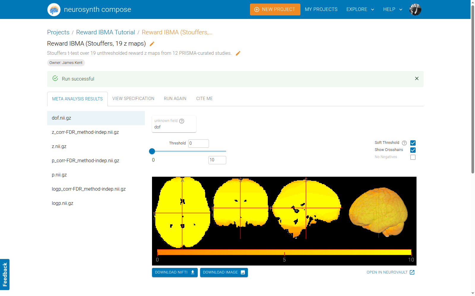
Seven output maps: z, p, logp, their FDR-corrected counterparts, and dof.

note

The file list defaults to dof.nii.gz with the metadata panel reading unknown field. That is the degrees-of-freedom map, not your result — click z_corr-FDR_method-indep.nii.gz.

At the default threshold (z > 2.58), almost the entire brain survives correction:

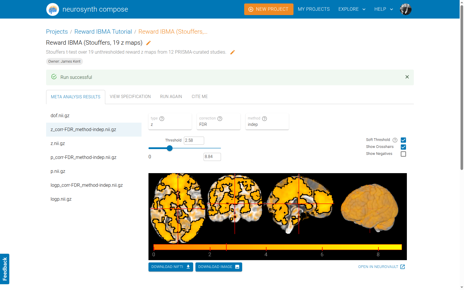
This is not a bug, and it is worth understanding. Stouffers over 19 unthresholded maps is extremely powerful, and unthresholded maps share a great deal of global structure, so the null hypothesis of exactly zero is rejected nearly everywhere.

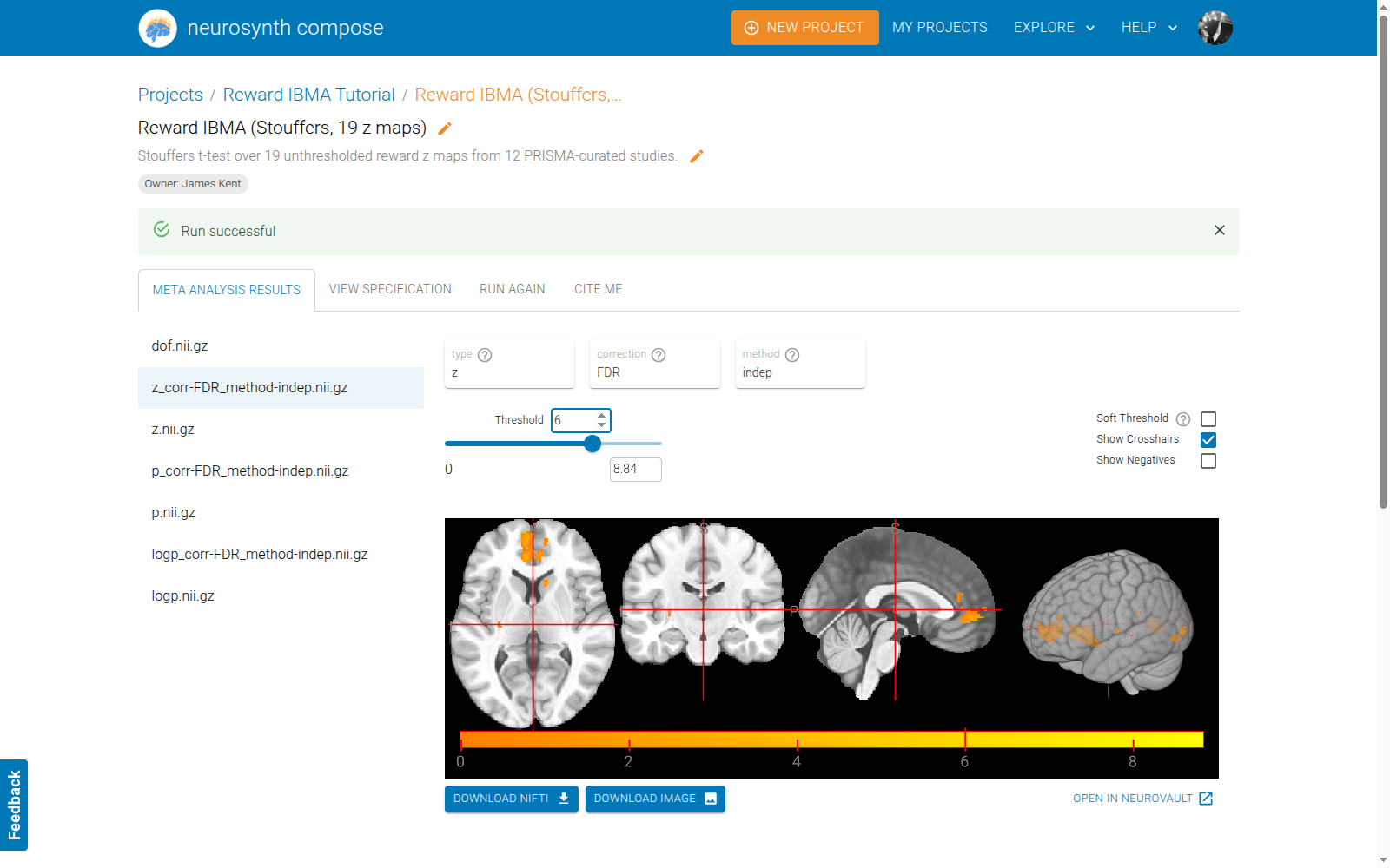
Raising the threshold to z > 6 with soft-thresholding off gives an interpretable figure:

Peaks

18 peaks were returned. The four dominant ones:

x	y	z	Z	Interpretation
10	10	−6	8.84	right ventral striatum / nucleus accumbens
−10	8	−8	8.58	left ventral striatum / nucleus accumbens
−6	54	−2	7.61	ventromedial prefrontal cortex / medial frontal pole
−6	42	2	7.00	anterior cingulate / vmPFC

Remaining peaks are an order of magnitude weaker (Z ≈ 1.8–2.8) and sit in temporal pole, lateral OFC and cerebellum. Two small negative peaks appear at (48, −28, −10) and (18, −40, 16).

---

14. Putting this in the context of the reward literature

The two strongest findings — bilateral ventral striatum and vmPFC/mOFC — are the two most reliably reported nodes of the human reward and valuation system, and recovering them is a good sign the pipeline behaved.

Bartra, McGuire & Kable (2013, NeuroImage) performed a coordinate-based meta-analysis of 206 subjective-value experiments and identified a "valuation system" centred on precisely these two regions, consistent across reward types and decision stages. Knutson & Greer (2008) localised anticipatory reward signals to ventral striatum, while outcome and value comparison recruit vmPFC more strongly. The striatal signal also aligns with the dopaminergic reward-prediction-error account (Schultz), which is directly relevant here since several included studies model prediction error explicitly.

The interesting observation is one of efficiency: 19 maps from 12 studies recovered the same core system that required ~200 studies to establish by coordinate-based methods. That is the theoretical case for IBMA in one result — each study contributes whole-brain evidence rather than a handful of supra-threshold peaks. It is a demonstration, not a replication, but it shows that even with limited data, the approach can yield robust and meaningful results. Go forth, try it, and see what you can discover (and report bugs!).